Ratio Outlier (Medcouple)

 Refer for Details:

https://drive.google.com/drive/folders/19IEg3V008AkBwT5UGrsXCL8N6It7BGc_?usp=sharing

Python Generic Code (Probability of Default Model Development, Validation and Testing):

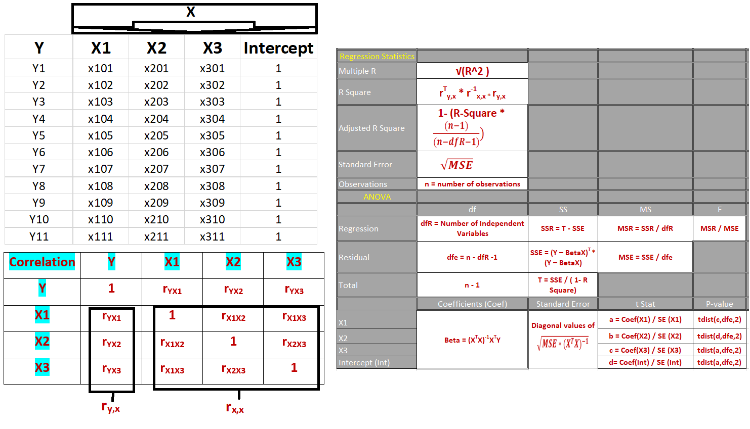
Python Generic Code (Probability of Default Model Development, Validation and Testing):
In the link below:

1- PD_Factors.csv: CSV with factors and required data
2- PD_Model_Generic_Python (Doc and PDF): Python generic code (as in steps)
3- PD_Estimate_Steps_Python: Steps in word as in Screenshot below

Bias & Variance Trade off:

 Errors of a model is decomposed into Noise, Bias and variance.

There is a tradeoff between a model's ability to minimize bias and variance.

Overfitting: Variance High; model is good in the training set but not in the testing data set. Low training error does not imply good expected performance: over‐fitting.
Underfitting: Bias High; Model is neither good in the training nor in the testing data.
Noise: The model is neither overfitting or underfitting, and the high MSE is simply due to the amount of noise in the dataset.

Error due to Bias: Actual Value – average (Predicted Value).
A high bias model characteristic:
1.   High training error.
2.   Validation error is similar in magnitude to the training error.
Error due to Variance:
 Is variability of a model prediction for a given data point. Repeating the entire model building process multiple times. The variance is how much the predictions for a given point vary between different realizations of the model.
A high variance model characteristic:
1.   Low training error
2.   Very high Validation error

Bayesian Inference

  Bayesian Inference

Update probability with new information (data).

Combining two distributions (Likelihood and Prior) into Posterior.

Posterior is used find the “best” parameters in terms of maximizing the posterior probability.

Steps:

i.            Prior: Choose a PDF to model i.e. the prior distribution P(θ).

ii.            Likelihood: Choose a PDF for P(X|θ). How the data X will look like given the parameter θ.

iii.            Posterior: Calculate the posterior distribution P(θ|X) and pick the θ that has the highest P(θ|X).

 

Calculate P(θ) & P(X|θ) for a specific θ and multiply them together. Pick the highest P(θ) * P(X|θ) among different θ’s.

 Posterior becomes the new prior. Repeat step 3 as you get more data.

Game

 

Beta Distribution

 Beta Distribution: the probability of success on any single trial as the random variable, and the number of trials n and the total number of successes in n trials as constants.

For the Binomial Distribution the number of successes X is a random variable and the number of trials N and the probability of success p on any single trial are parameters (i.e. constants).

Standard Deviation of Pooled Set vs Subsets (Unequal Size):

 

Identifying Outlier in Ratio detection for skewed distribution

https://docs.google.com/spreadsheets/d/1gBjuMYN_pRLu2MfNU0WW9zzsq5EMIN6d/edit?usp=sharing&ouid=115594792889982302405&rtpof=true&sd=true:

 

 

Asymptotic Single Risk Factor Model (ASRF):

 Key assumptions: asymptoticity, a single risk factor, and normality.

PD assumptions and violations:

Probability of observing D defaults over N (total number of exposures in the credit portfolio) independent random draws follows a binomial distribution.
PD ASRF model Binomial Distribution assumptions:
  i.  Each asset in the rating grade has default probability P.
 ii.  Each pair of assets has default correlation ρ
iii.  The conditional correlation between any two assets is constant even if the number of defaults increases.
iv.   Normal distribution assumption for the systematic factor
 
ASRF model assumptions may get violated:

Assumptions (i) and (ii):
Let x1, ..,xn be random indicator variables representing the default behavior of the assets where xj =1 indicates the default of asset j. Define as the probability of default of asset j given that assets 1 to j-1 are known to have defaulted.
Assumptions (i) and (ii) imply that:
P1 = P and P2 = P + (1 - P )*ρ
When assets are independent ρ = 0 than these assumptions lead to the Binomial distribution with Pj = P.
However, If ρ > 0, then x1, ..,xn are not independent than the assumption of Binomial distribution is violated.
Assumption (iii):
If the conditional correlation between any two assets increase as the number of defaults increases will lead to increase in default probability.
The increasing default probability given other defaults results in fatter tails of the Correlated Binomial distribution. Contrast assumption (3) with the Binomial distribution where the independence assumption implies that ρj = ρ for all j=1,..,n assets
 
Assumption (iv):
Systematic factor may follows an autoregressive process.

Modeling Low Default Portfolio Dependent Case:

 Modeling Low Default Portfolio Dependent Case:

VASCIEK MODEL: Dependence between the default is explained by by Vasicek model.

By using conditional probability from the Vasicek model in the case where there are no defaults, the probability of default is the solution of below equations:

Low Default Portfolio (PD)

 Modeling Low Default Portfolio (Independent Default Events):

Pluto and Tasche method for calculating probability of default for portfolios with none or very few observations of defaults.
One-sided upper confidence bound as an estimator of PD.

Assumptions:
- n >0 borrowers in the portfolio.
- At the end of the observation period 0≤ d < n defaults are observed among the n borrowers.
- Default events are independent, hence the number of defaults in a portfolio is binomially distributed:
nCr * p^r * ((1-p)^(n-r)
n is the total number of borrowers, r is the total number of defaults and p is the probability of default.
PD to be logical, it should have the following characteristic:
p1 <= p2 <=p3 <=p4..........
It also means that p1=p2=p3=p4=p5...... In this scenario, all the 500 borrowers belong to the same risk characteristic, i.e. homogenous borrowers.

E.g: 

https://drive.google.com/file/d/1OmGmQV-AsYPsfdRYowSy1bkZArgEFMvN/view?usp=sharing

Matrix Format of Regression Output

 Matrix Format of Regression Output